Chapter 2: Signal and System Foundations for Medical Imaging
2.1 Introduction
Mathematical functions are fundamental tools used to describe and analyze systems in bioimaging and biomedical signal processing. Imaging modalities such as magnetic resonance imaging (MRI), ultrasound, and optical imaging rely on mathematical models to relate physical inputs to measurable outputs. By representing these relationships using functions, complex biological and physical processes can be systematically analyzed and optimized.
In bioimaging, signals and images are often interpreted as functions of time, space, or frequency. Understanding how these functions behave allows engineers and scientists to design imaging systems that accurately capture biological information. This chapter introduces the core concepts of functions and mapping, followed by an exploration of linear and sinusoidal functions, which are widely used in bioimaging and signal processing applications.
2.2 Functions and System Definitions
A function is a mathematical relationship that assigns exactly one output value to each input value. This concept is especially important when describing systems that transform an input signal into an output signal. In bioimaging, systems can include physical devices, biological tissues, or computational algorithms that operate on data.
A system can be modeled mathematically as a function that processes an input to produce an output. For example, an optical imaging system maps reflected light intensity from tissue to a digital image, while an MRI system converts electromagnetic signals into spatial information. Representing these systems as functions allows their behavior to be predicted, analyzed, and improved using mathematical techniques.
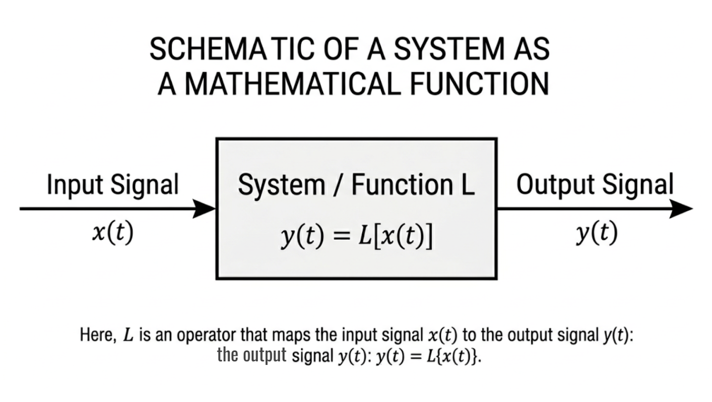
Figure 2.1: Representation of a system as a mathematical function mapping an input signal to an output signal. |
2.3 Domain, Range, and Mapping
The domain of a function is the set of all input values for which the function is defined. In bioimaging applications, the domain may represent time intervals, spatial coordinates, or frequency ranges over which measurements are taken. Ensuring that inputs remain within the domain is critical for accurate and stable system performance.
The range of a function consists of all possible output values produced when the function is applied to the domain. In imaging systems, the range may correspond to signal amplitudes, pixel intensities, or voltage levels. Understanding the range helps prevent issues such as saturation, clipping, or loss of information in measurement systems.
A mapping describes how each element of the domain is associated with an element of the range. In bioimaging systems, this mapping defines how physical quantities such as tissue properties or electromagnetic signals are converted into measurable data. A valid function ensures that each input maps to a single output, preserving consistency and interpretability in system design.
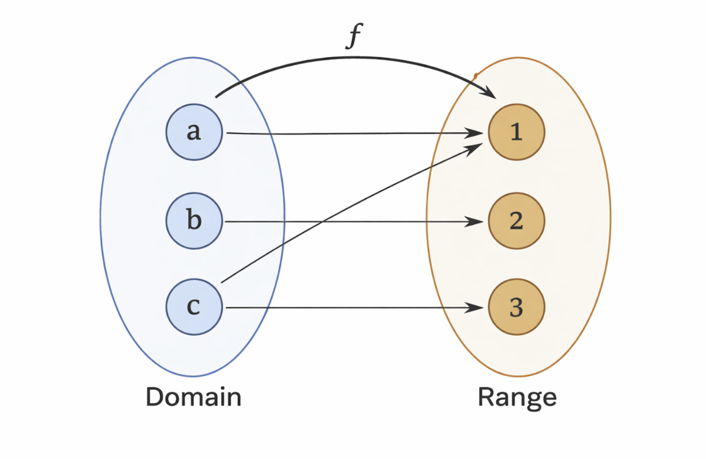
Figure 2.2: Illustration of a function mapping elements from a domain to a range. |
2.4 Linear Functions
A linear function is a function in which the output changes proportionally with the input. It is commonly expressed in the form $f(x) = mx + b$, where the slope $( m )$ determines the rate of change and the intercept $( b )$ defines the output when the input is zero. Linear functions are among the simplest mathematical models used in engineering and science.
In bioimaging systems, linear functions are frequently used to model sensor responses and signal amplification. For example, an increase in light intensity detected by a photodetector may produce a proportional increase in electrical voltage within a linear operating range. Linear models are particularly useful because they allow for straightforward analysis and interpretation of system behavior.
Many imaging systems are designed to operate in a region where their response is approximately linear. This assumption enables the use of linear system theory, including superposition and scaling, which greatly simplifies signal processing and image reconstruction. Although real systems may exhibit nonlinear behavior, linear approximations remain a powerful and widely used tool.
2.5 Sinusoidal Functions
Sinusoidal functions describe oscillatory behavior and are characterized by smooth, repeating waveforms. These functions are typically expressed using sine or cosine functions, which include parameters that control amplitude, frequency, and phase. Sinusoidal behavior is commonly observed in natural and engineered systems.
In signal processing, sinusoidal functions are fundamental because they form the building blocks of more complex signals. Many biomedical signals, including electromagnetic waves used in imaging systems, exhibit sinusoidal properties. Techniques such as Fourier analysis rely on the fact that any complex signal can be represented as a combination of sinusoidal components.
In bioimaging applications, sinusoidal functions are used to encode, transmit, and analyze information. For example, MRI systems use oscillating magnetic fields and radiofrequency signals that are inherently sinusoidal. Understanding sinusoidal functions is therefore essential for analyzing frequency content, designing filters, and interpreting imaging data.
2.6 Comparison of Linear and Sinusoidal Functions
Linear and sinusoidal functions serve different but complementary roles in bioimaging and signal processing. Linear functions are primarily used to describe proportional relationships and system responses, while sinusoidal functions are used to model periodic and frequency-based behavior. Both types of functions are essential for a complete understanding of imaging systems.
Linear functions are especially useful in modeling amplification, attenuation, and calibration processes. Sinusoidal functions, on the other hand, are critical for understanding signal modulation, wave propagation, and spectral analysis. Together, these functions provide a mathematical framework for describing how bioimaging systems acquire and process data.
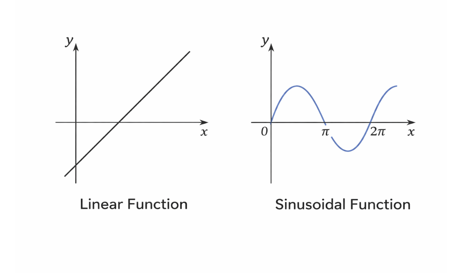
Figure 2.3: Comparison of linear and sinusoidal functions commonly used in signal processing and imaging. |
2.7 Taylor Expansion
The Taylor expansion is a mathematical technique used to approximate complex functions using a sum of simpler polynomial terms. Rather than working directly with a complicated function, the Taylor expansion represents the function as a series of terms that are easier to analyze and compute. This approach is especially valuable in engineering and bioimaging, where exact analytical expressions may be difficult or impossible to evaluate.
A Taylor expansion begins at a specific point, often called the expansion point or operating point. The first term in the expansion is a constant equal to the value of the function at that point. This constant term provides a baseline approximation and represents the function’s output when the input is exactly at the expansion point.
The next term in the Taylor expansion is a linear term, which depends on the first derivative of the function evaluated at the same point. This term accounts for how the function changes in response to small variations in the input. In practical systems, this linear term often dominates the behavior near the operating point and forms the basis for linear approximations used in signal processing and system modeling.
Higher-order terms are then added to improve the accuracy of the approximation. The quadratic term depends on the second derivative of the function and captures curvature in the function’s behavior. Additional terms involving higher-order derivatives can be included as needed, allowing the approximation to more closely match the original function over a wider range of inputs.
In bioimaging and biomedical signal processing, Taylor expansions are commonly used to simplify nonlinear system behavior. Small deviations around an operating point can often be analyzed using only the constant and linear terms, resulting in a linearized model. This technique enables efficient analysis of imaging systems, noise behavior, and signal distortions while maintaining sufficient accuracy for practical applications.
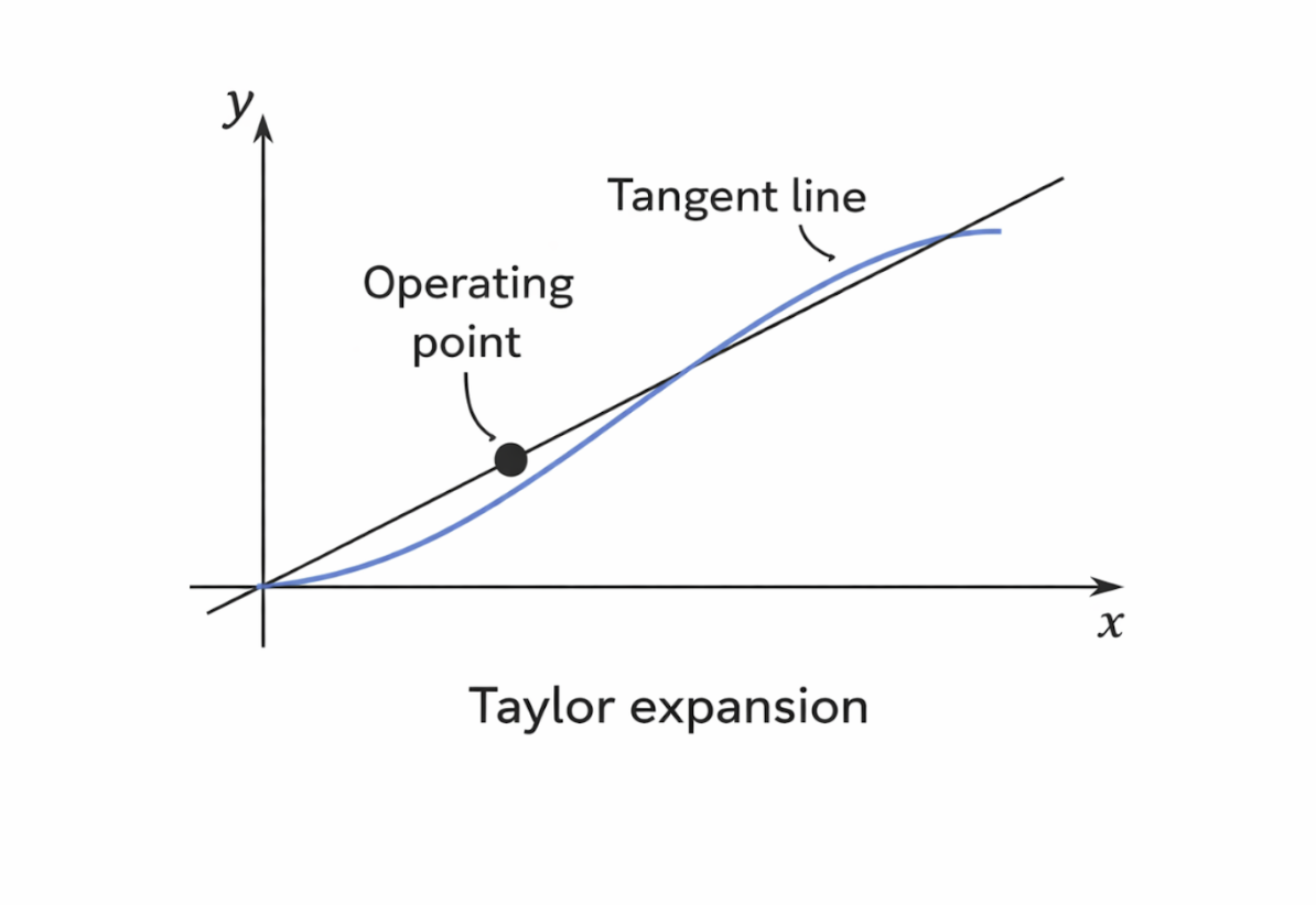
Figure 2.4: Local linear approximation of a nonlinear function using a Taylor expansion around an operating point. |
2.8 Linear Functions in One and Two Dimensions
Linear functions are among the most important mathematical tools used in engineering and medical imaging because of their simplicity and interpretability. In one dimension, a linear function describes how a single input variable maps to a single output variable, typically in the form $f(x) = mx + b$. This type of function is commonly used to model relationships such as signal amplitude as a function of time or sensor output as a function of input intensity.
Two-dimensional linear functions extend this concept by mapping inputs from a two-dimensional domain to outputs. In medical imaging, two-dimensional linear relationships often arise when modeling images, which can be represented as functions of spatial coordinates $(x,y)$. Linear models in two dimensions are frequently used in image formation, filtering, and reconstruction algorithms.
Linear functions are easy to analyze because their behavior is predictable and well understood. They obey principles such as superposition and scaling, which allow complex problems to be broken down into simpler components. Additionally, linear functions are fast to compute, making them especially well suited for real-time imaging applications where large amounts of data must be processed efficiently.
In medical imaging, linear approximations are widely used even when systems are not perfectly linear. Many imaging devices are designed to operate within a range where their response is approximately linear, enabling accurate modeling and reconstruction. This reliance on linear functions forms the mathematical foundation for many imaging techniques, including image filtering, noise reduction, and tomographic reconstruction.
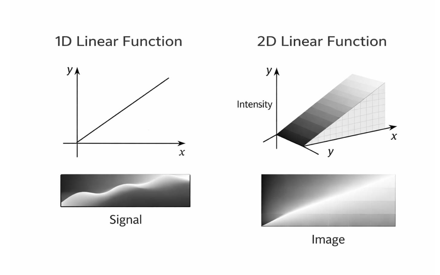
Figure 2.5: One-dimensional signals and two-dimensional images represented as linear functions. |
2.9 Systems, Inputs, and Outputs
A system is a process that takes an input, performs some operation, and produces an output. In mathematical terms, a system can be represented as an operator that acts on an input signal or function. This abstraction allows physical devices, biological processes, and computational algorithms to be described using a common mathematical framework. If (v(t)) represents an input signal and (w(t)) represents an output signal, a system can be written as
\[w(t) = L(v(t))\]where (L) denotes the system operator. In cases where time dependence is not explicitly emphasized, the system may be written more compactly as:
\[w = L(v)\]This notation highlights that the output is determined entirely by how the system processes the input.
In medical imaging systems, inputs may include electromagnetic signals, acoustic waves, or electrical measurements, while outputs may be digital images or reconstructed signals. The system performs a sequence of physical and computational operations that transform the input into a usable form. Understanding the relationship between inputs and outputs is essential for designing, analyzing, and improving imaging systems.
Mathematics and tomographic scanners are tightly integrated within these systems. Tomographic imaging modalities rely on mathematical models to reconstruct internal structures from external measurements. By treating the scanner as a system and using linear operators to describe its behavior, engineers can develop algorithms that accurately convert raw data into clinically meaningful images.
2.10 Measurement Systems
A measurement system is a system designed to quantify an unknown physical quantity by comparing it to a known reference. The reference provides a standard against which the unknown value can be evaluated, allowing the measurement to be expressed in meaningful units. This comparison process is fundamental to all scientific and engineering measurements.
For example, measuring electrical voltage involves comparing an unknown voltage to a calibrated reference within a voltmeter. Similarly, measuring tissue temperature requires comparing thermal energy emitted by tissue to a known temperature scale. In each case, the accuracy of the measurement depends on the quality of the reference and the reliability of the system performing the comparison.
Measurement systems are essential in biomedical engineering because biological quantities cannot be directly observed in numerical form. Instead, sensors and instruments convert physical or chemical properties into measurable signals. These systems form the foundation upon which imaging systems and diagnostic tools are built.
2.11 Imaging Systems
An imaging system is a specialized type of measurement system that produces a spatial representation of an object or region of interest. Rather than measuring a single value, imaging systems measure variations across space and map them into an image. Each point in the image corresponds to a specific location in the object being measured.
Magnetic resonance imaging (MRI) scanners are a prominent example of imaging systems in medicine. In an ideal imaging system, a single point in the reconstructed image corresponds exactly to a single point in the body. This precise correspondence allows anatomical structures and physiological features to be accurately visualized.
In practice, imaging systems are imperfect, and their limitations affect image quality. A low-quality imaging system may blur features, causing distinct structures to appear smeared or indistinct. This blurring is a characteristic of the system itself and reflects how the system processes and transforms the measured signals. Understanding these system characteristics is essential for interpreting images and improving imaging performance.
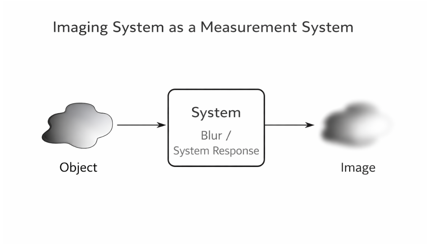
Figure 2.6: Imaging system as a measurement process mapping object properties to a reconstructed image. |
2.12 Control Systems
A control system is a type of system that does not stop after producing an output, but instead uses that output as feedback to modify its own behavior. In a control system, the output is continuously monitored and compared to a desired reference or goal. Any difference between the actual output and the desired output is used to adjust the system’s operation.
This feedback mechanism allows control systems to maintain stability and accuracy even in the presence of disturbances or changing conditions. For example, a thermostat-controlled heating system measures the current room temperature and compares it to a set temperature. If the temperature deviates from the desired value, the system automatically adjusts the heating output to correct the difference.
Control systems are widely used in biomedical and engineering applications because they enable precise regulation of complex processes. In medical devices, feedback control can be used to regulate drug delivery, maintain stable physiological conditions, or adjust imaging parameters in real time. The ability to self-correct makes control systems more robust and reliable than open-loop systems.
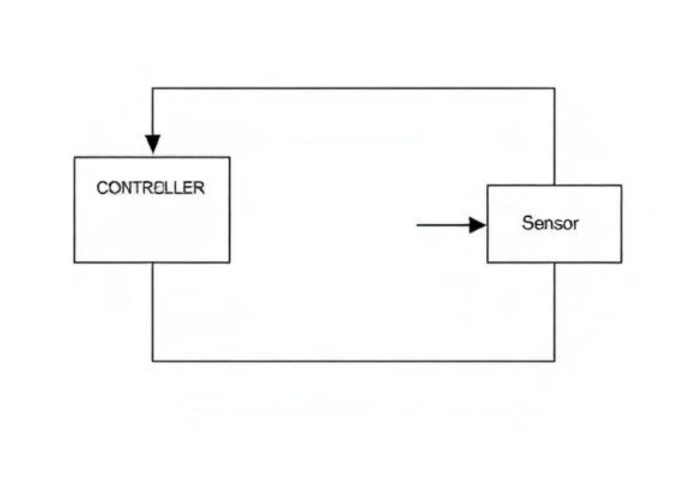
Figure 2.7: A closed-loop control system in which the output is continuously measured and fed back to adjust system behavior. |
2.13 Robotic Systems
A robotic system is a specialized type of control system that integrates sensing, computation, and actuation to interact with its environment. In addition to feedback control, robotic systems often incorporate a level of machine intelligence that allows them to make decisions and adapt their behavior. These systems typically maintain a three-dimensional model of the surrounding world, which helps them navigate and perform tasks accurately.
In real-world applications, robotic systems are used in manufacturing, exploration, and healthcare. For example, industrial robots adjust their motion based on sensor feedback to assemble products with high precision. Autonomous vehicles use sensors and control algorithms to adapt to changing road conditions and avoid obstacles.
In medicine, robotic systems are increasingly used alongside medical imaging to guide surgical procedures. Imaging systems provide spatial information about the patient’s anatomy, while the robotic system uses this information to position instruments accurately. By combining imaging data, feedback control, and intelligent decision-making, robotic systems enhance precision, reduce invasiveness, and improve patient outcomes during complex surgical interventions.
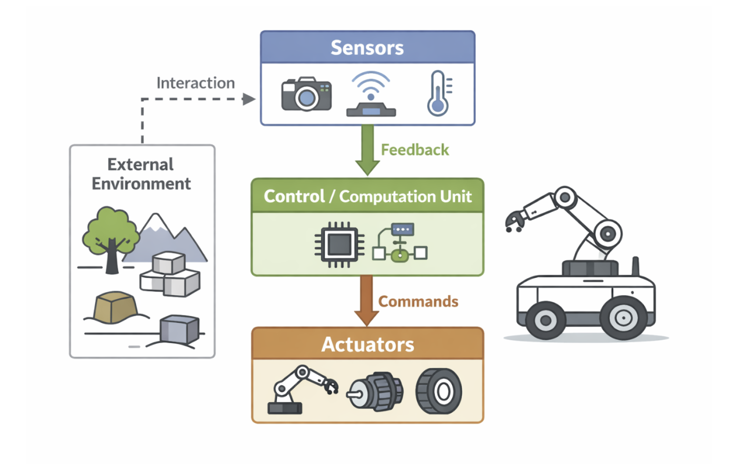
Figure 2.8: Core components of a robotic system integrating sensing, computation, actuation, and feedback control. |
2.14 Neurological Systems
The neurological system is a complex biological system responsible for sensing, processing, and responding to information from the environment. Neurons receive input in the form of chemical or electrical signals and transmit electrical impulses that propagate through neural networks. These signals enable essential functions such as perception, movement, cognition, and regulation of internal bodily states.
At the cellular level, neurons act as information-processing units that integrate multiple inputs before generating an output signal. This process closely resembles engineered systems in which inputs are transformed through defined mechanisms to produce outputs. In bioimaging and neuroscience, measuring and visualizing neural activity is critical for understanding how information flows through the nervous system.
The neurological system does not operate in isolation but interacts continuously with other systems in the body. Sensory input, motor output, and internal feedback loops work together to maintain coordinated function. This system-level perspective is essential for studying brain function and neurological disorders.
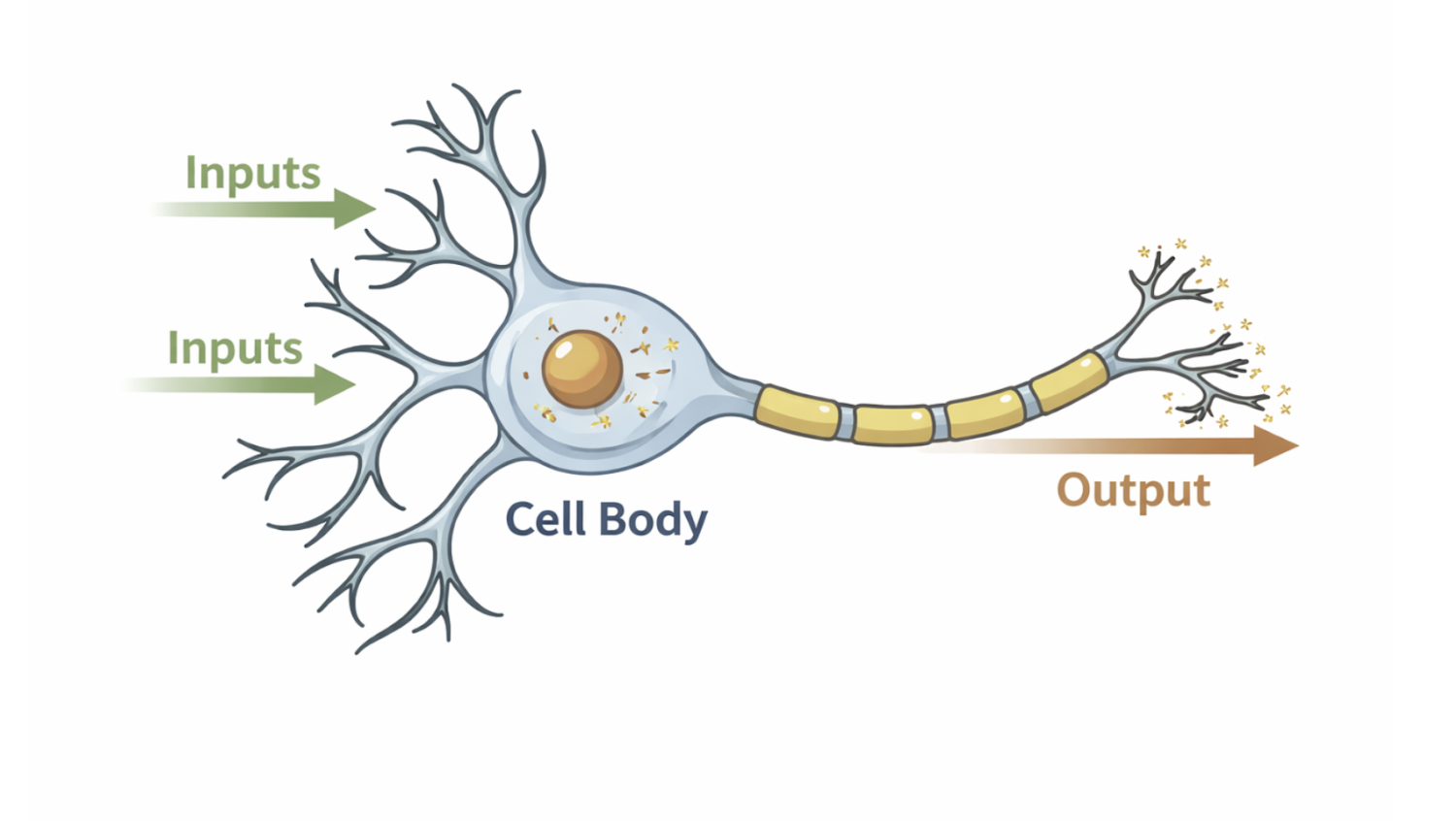
Figure 2.9: A neuron modeled as an information-processing system that integrates multiple inputs to produce an output signal. |
2.15 The Human Body as an Interconnected System
The human body can be understood as an interconnected system composed of multiple levels of organization. These levels range from genes and cells to tissues, organs, and large-scale systems such as the circulatory, respiratory, and neurological systems. Each level interacts with others, creating a highly integrated and dynamic biological network.
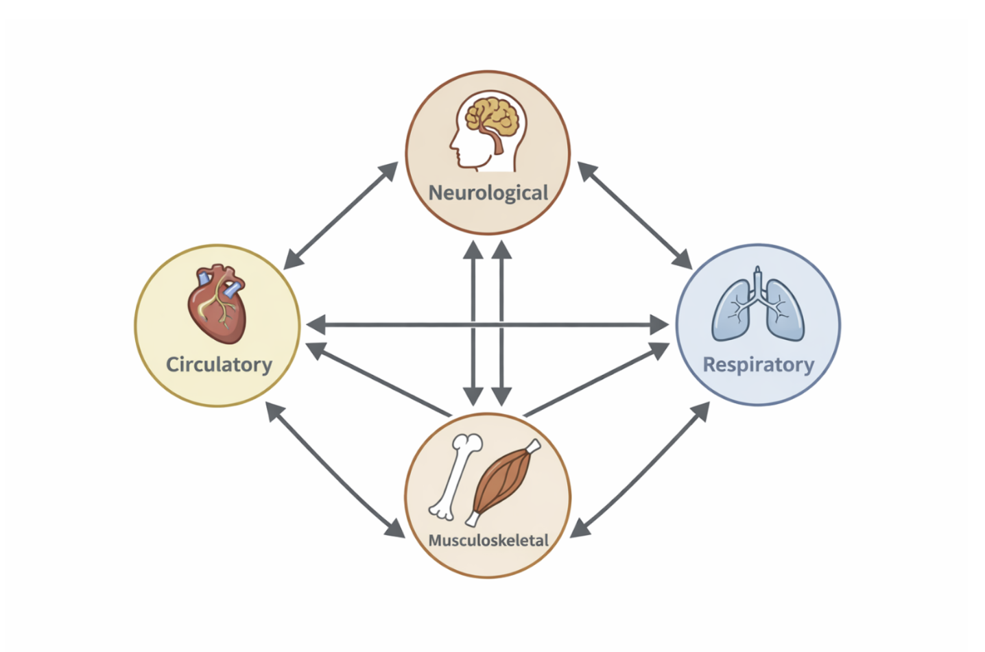
Figure 2.10: The human body viewed as an interconnected system of interacting subsystems across multiple scales. |
Biomedical engineering and bioimaging focus on studying the body as a collection of interacting components rather than isolated parts. Changes at the molecular or cellular level can propagate upward to affect organ function and overall health. Imaging technologies play a crucial role in visualizing these interactions across scales, allowing researchers and clinicians to observe structure and function simultaneously.
Viewing the human body as a system enables more accurate modeling, diagnosis, and treatment of disease. Systems-based approaches support advances such as personalized medicine, functional imaging, and targeted therapies. This perspective aligns closely with the mathematical and system-theoretic concepts introduced earlier in this chapter.
2.16 Convergence of Human and Robotic Systems
The distinction between human biological systems and artificial engineered systems is becoming increasingly blurred. Advances in technology have enabled direct interactions between the human nervous system and machines, particularly in the fields of brain–machine interfaces and neural prosthetics. These developments allow artificial systems to receive input from, and deliver output to, biological systems.
Emerging fields such as neuro-inspired artificial intelligence and embodied intelligence draw inspiration from how humans sense, learn, and adapt to their environment. In these systems, intelligence is not purely computational but is shaped by interaction with the physical world. This mirrors how human cognition is deeply connected to sensory input, motor control, and feedback.
In biomedical applications, robotic and artificial systems are increasingly integrated with medical imaging and neural data. Examples include brain-controlled prosthetic limbs and image-guided robotic surgery systems. As these technologies continue to develop, understanding both human and artificial systems through a shared systems framework becomes essential for advancing medicine and healthcare.
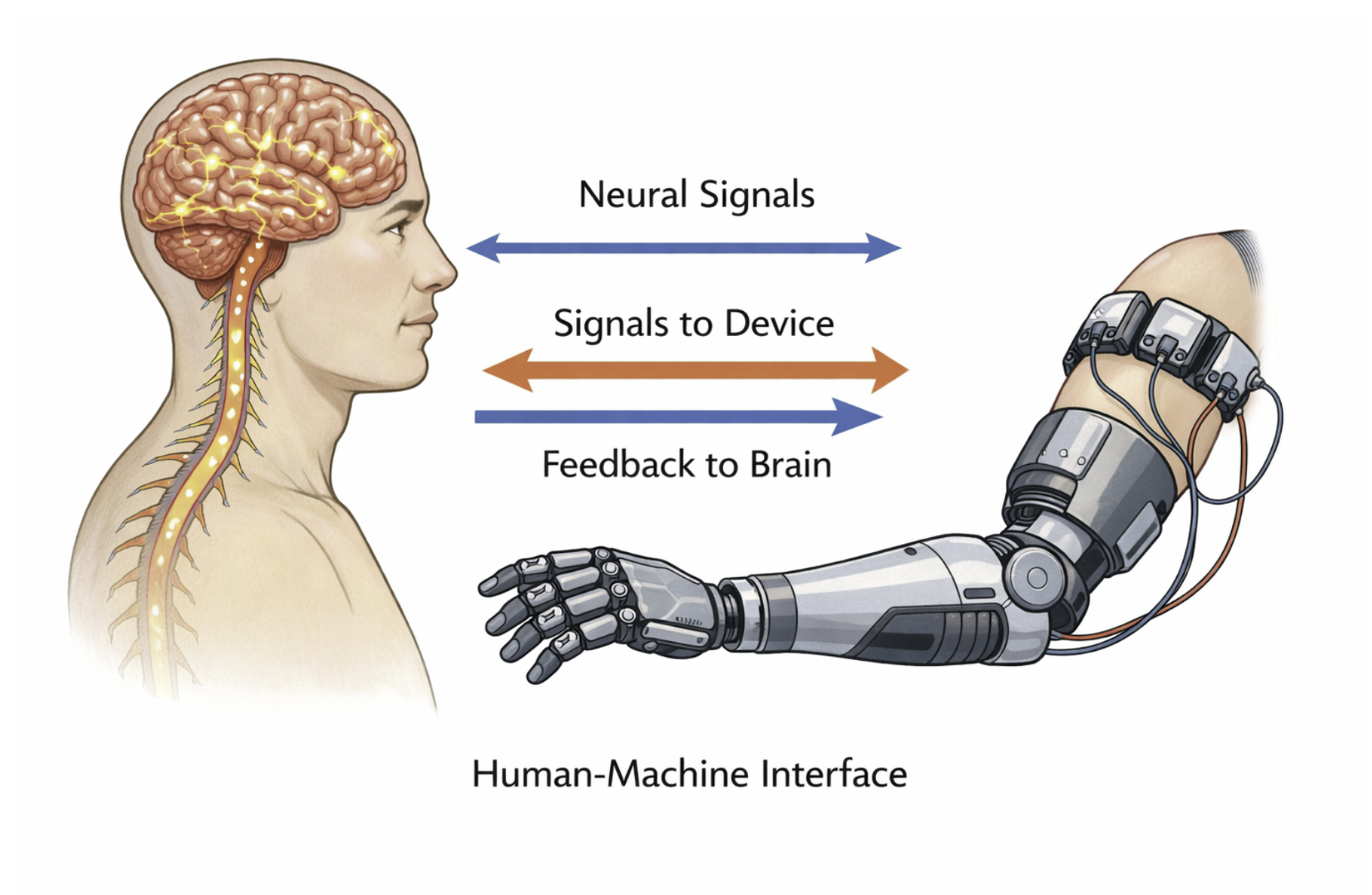
Figure 2.11: Conceptual representation of interaction between biological systems and engineered systems through neural interfaces. |
2.17 Linear Systems
A system is defined as linear if it satisfies two fundamental properties: additivity and homogeneity. These properties describe how the system responds to combinations and scalings of inputs. Linear systems are central to biomedical signal processing and medical imaging because they are mathematically tractable and allow powerful analytical tools to be applied.
Mathematically, if a system is represented by an operator (L) acting on an input signal (v(t)), linearity ensures predictable and consistent behavior. This predictability is essential in imaging systems, where signals are often decomposed, processed, and recombined. Many imaging and reconstruction algorithms are explicitly designed under the assumption of linearity.
An important consequence of linearity is that a linear system must produce zero output when given zero input. If an input signal contains no energy or information, the system cannot generate output on its own. This condition follows directly from the properties of additivity and homogeneity.
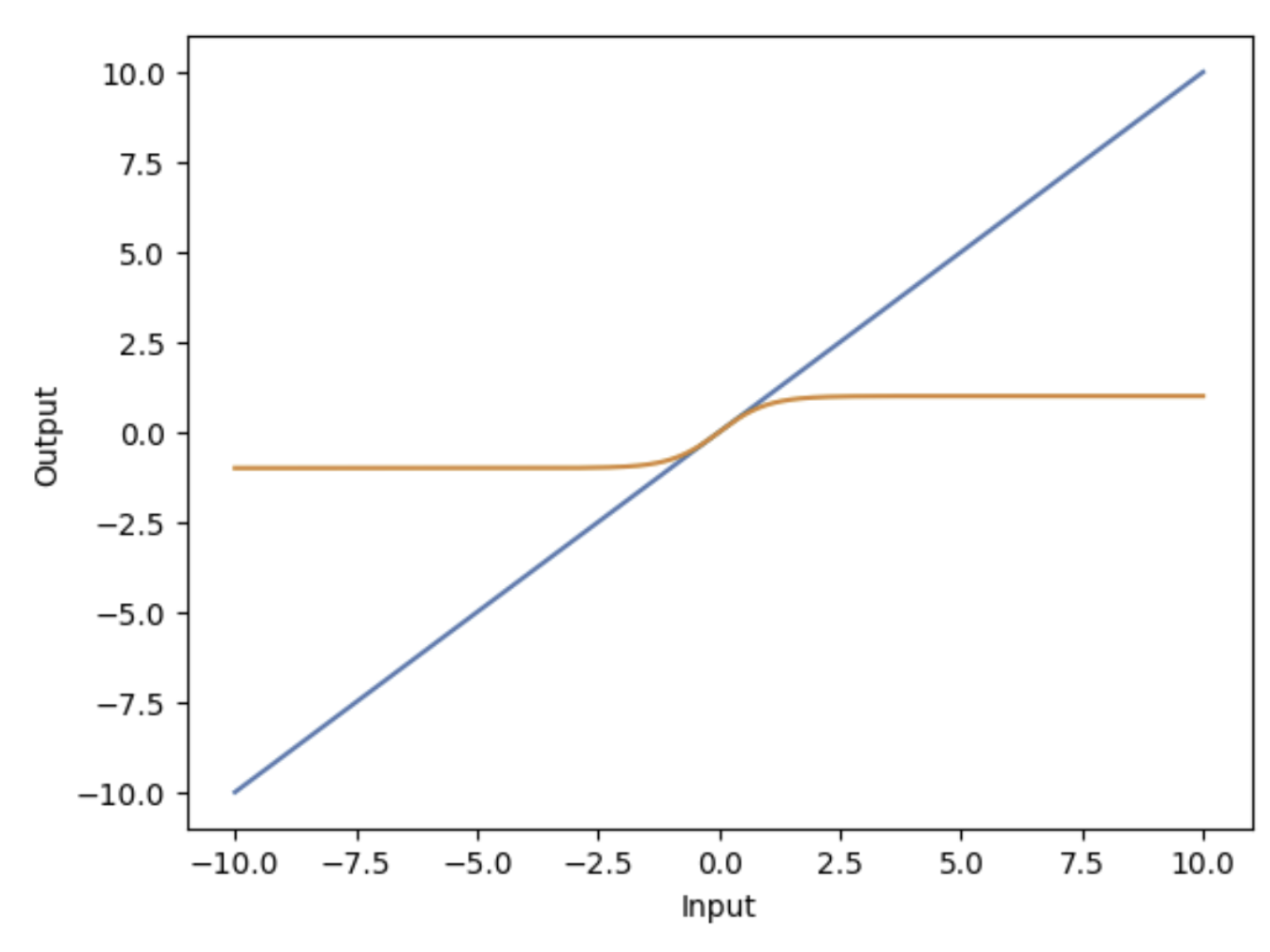
Figure 2.12: Comparison of linear and nonlinear system responses illustrating proportional versus nonlinear behavior. |
2.18 Additivity
Additivity describes how a system responds to the sum of two inputs. A system is additive if the response to a combined input equals the sum of the individual responses. In mathematical terms, this property is expressed as
\[L(v_1(t) + v_2(t)) = L(v_1(t)) + L(v_2(t))\]
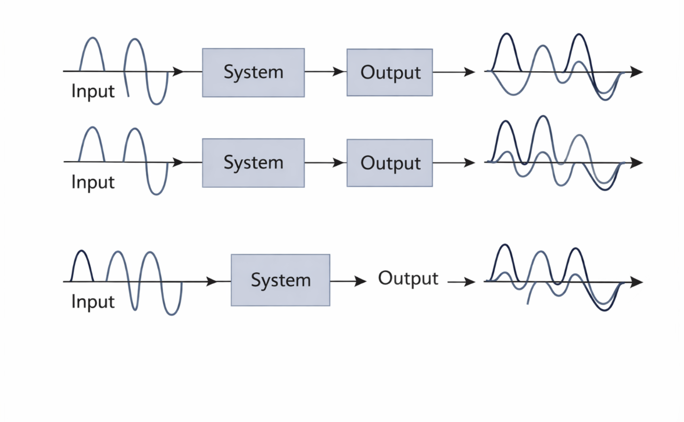
Figure 2.13: Illustration of additivity: the response to a sum of inputs equals the sum of the individual responses. |
This concept can be illustrated using function notation. If an input function (f_1(x)) is processed by a system (H) to produce an output (K_1(x)), and another input (f_2(x)) produces an output (K_2(x)), then the combined input(f_1(x) + f_2(x)) must produce the combined output (K_1(x) + K_2(x)). Symbolically:
\[\begin{align*} f_1(x) &\rightarrow H[f_1(x)] \rightarrow K_1(x), \\ f_2(x) &\rightarrow H[f_2(x)] \rightarrow K_2(x), \\ f_1(x) + f_2(x) &\rightarrow H[f_1(x) + f_2(x)] \rightarrow K_1(x) + K_2(x). \end{align*}\]Additivity allows complex inputs to be broken into simpler components that can be analyzed independently. Each component is processed separately, and the individual results are then combined to understand the system’s overall response. In medical imaging, this principle is critical for image reconstruction, where measured signals are often decomposed into contributions from different spatial locations or tissue properties.
2.19 Homogeneity
Homogeneity describes how a system responds when an input is scaled by a constant factor. A system is homogeneous if scaling the input by a scalar α\alphaα results in the output being scaled by the same factor. This property is expressed mathematically as:
\[L(\alpha v(t)) = \alpha L(v(t))\]
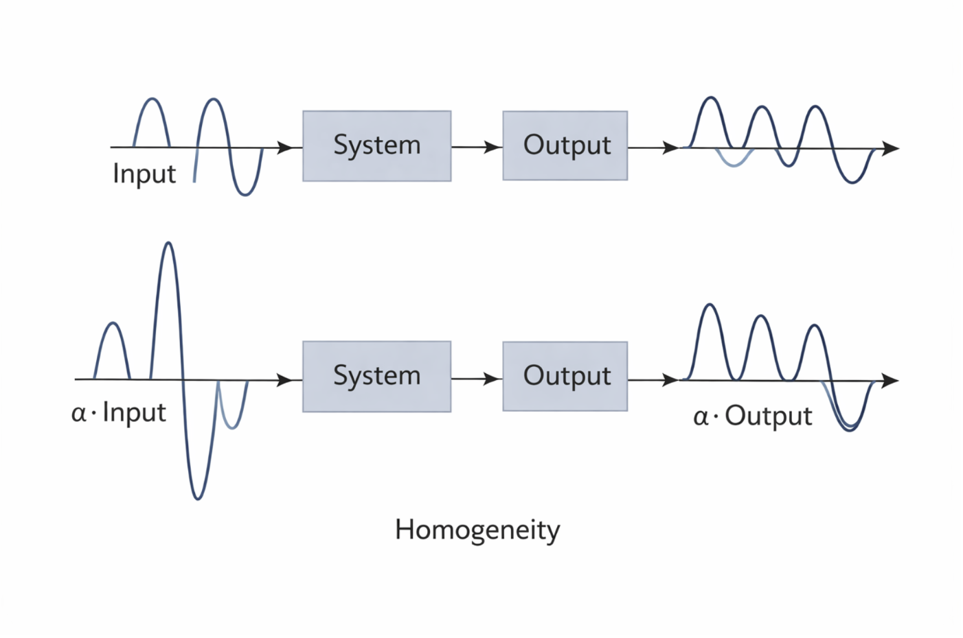
Figure 2.14: Illustration of homogeneity: scaling the input scales the output by the same factor. |
Using function notation, if an input (f_1(x)) produces an output (K_1(x)), then scaling the input by a constant (a_1) must scale the output accordingly. This relationship can be written symbolically as:
\[\begin{align*} f_1(x) &\rightarrow H[f_1(x)] \rightarrow K_1(x), \\ a_1 f_1(x) &\rightarrow H[a_1 f_1(x)] \rightarrow a_1 K_1(x), \end{align*}\]which implies:
\[H[a_1 f_1(x)] = a_1 H[f_1(x)].\]Homogeneity ensures that the system preserves relative signal strength. In medical imaging, this means that doubling the signal intensity from tissue should double the measured response, assuming the system is operating within its linear range. This property is essential for accurate quantitative imaging.
2.20 Superposition and Zero Input Response
The superposition principle states that the response of a linear system to a weighted sum of inputs equals the same weighted sum of the individual responses. This principle follows directly from the combined application of additivity and homogeneity. Together, these properties allow linear systems to handle complex inputs by decomposing them into simpler signals.
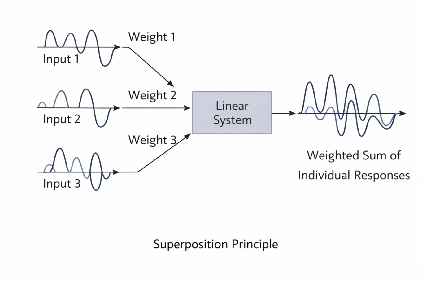
Figure 2.15: Superposition principle in linear systems: complex inputs can be decomposed into simpler components whose responses add linearly. |
A direct consequence of homogeneity is that if the input to a linear system is zero, the output must also be zero. Setting the scalar (\alpha = 0) in the homogeneity condition yields:
\[L(0 \cdot v(t)) = 0 \cdot L(v(t)) = 0\]This confirms that linear systems cannot generate output without an input. When dealing with infinite sums of input components, linearity requires that the resulting infinite sum of outputs must converge. This condition ensures that the system’s response remains finite and physically meaningful. In imaging systems, convergence is critical when reconstructing images from large or continuous datasets.
2.21 Relationship Between Additivity and Homogeneity
Additivity and homogeneity are closely related but represent distinct aspects of linearity. Neither property alone is sufficient to guarantee that a system is linear. Additivity describes how the system handles multiple inputs, while homogeneity describes how it handles scaling.
Together, additivity and homogeneity define linearity, and both are required as separate conditions. However, when both properties hold, they combine to produce the superposition principle. In practice, linear systems are tested by verifying both conditions rather than attempting to derive one from the other.
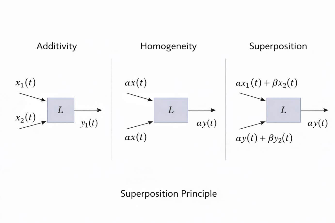
Figure 2.16: Illustration of additivity, homogeneity, and their combination into the superposition principle for linear systems. |
In biomedical signal processing and medical imaging, verifying linearity allows engineers to apply powerful mathematical tools such as convolution, Fourier analysis, and inverse problem techniques. These tools form the foundation of image formation, reconstruction, and enhancement algorithms used throughout modern medical imaging.
2.22 Equivalence of Additivity and Homogeneity in Continuous Systems
In general, linearity is defined by the two separate conditions of additivity and homogeneity. However, in the special case of continuous systems, these two properties are not independent. Under continuity assumptions, one property can be derived from the other, meaning that additivity and homogeneity become mathematically equivalent.
This equivalence is important in theoretical system analysis because it simplifies the conditions required to establish linearity. Instead of verifying both properties independently, it is sufficient to verify one property along with continuity. This result has practical implications for modeling physical and imaging systems, which are often assumed to behave continuously.
|
Figure 2.16: In continuous systems, additivity and homogeneity are mathematically equivalent under continuity assumptions. |
2.23 Homogeneity Implies Scaling Properties
Consider a function (f(x)) that satisfies homogeneity, meaning that for any scalar (n),
\[f(nx) = n f(x)\]
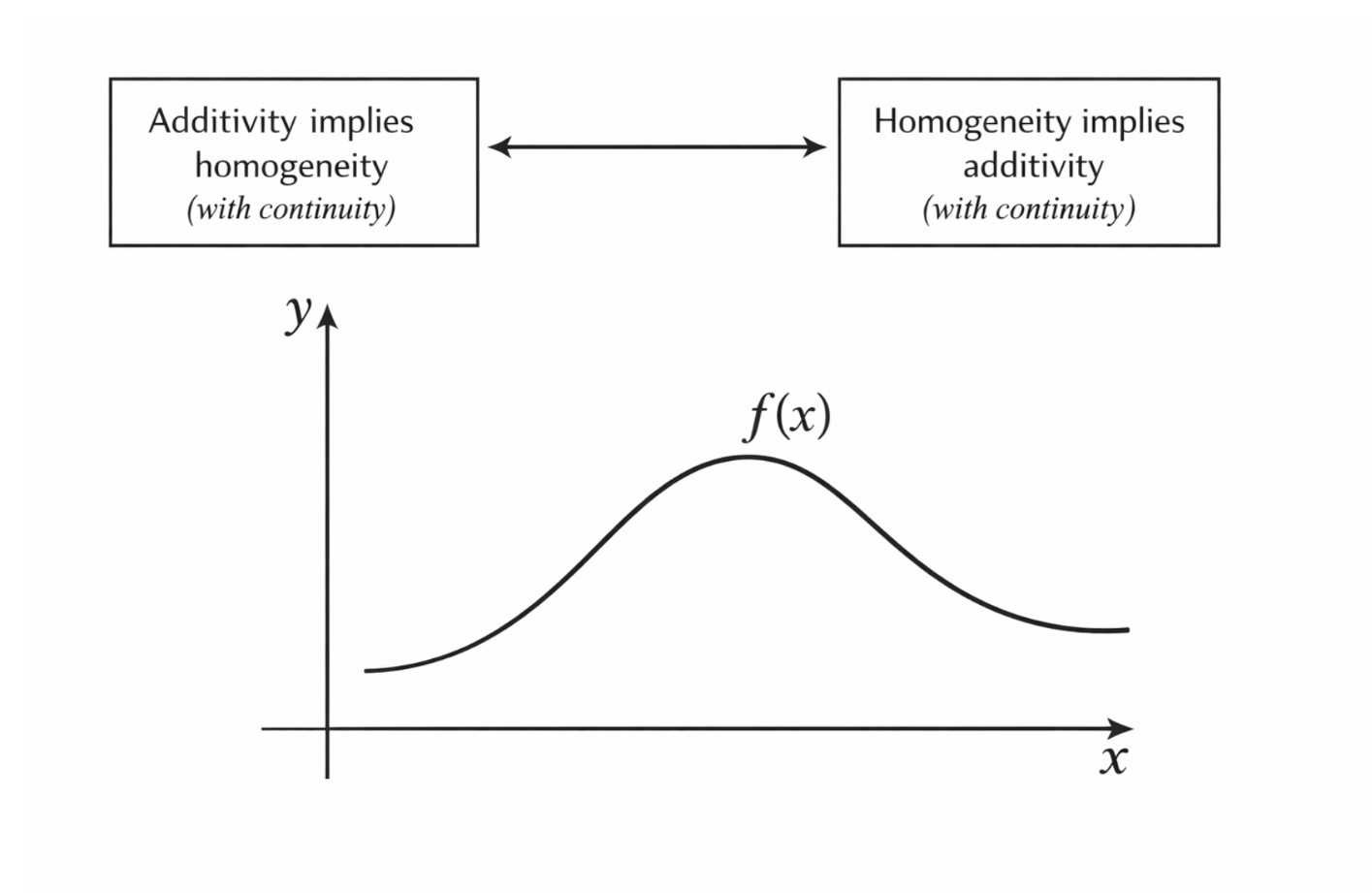
Figure 2.17: Homogeneity illustrated through proportional scaling of both input and output. |
This equation expresses the idea that scaling the input by a factor (n) scales the output by the same factor. This is the defining characteristic of homogeneity.
From this property, additional scaling relationships can be derived. For example, the function value at (x) can be written as:
\[f(x) = f\left(m \cdot \frac{x}{m}\right) = m f\left(\frac{x}{m}\right),\]which implies:
\[f\left(\frac{x}{m}\right) = \frac{1}{m} f(x).\]This result shows that homogeneity applies not only to integer scaling but also to fractional scaling, provided the system behaves continuously.
Homogeneity also imposes constraints on the function’s behavior at the origin. Using additivity at zero:
\[f(0) = f(x + (-x)) = f(x) + f(-x),\]which implies:
\[f(-x) = -f(x).\]This result confirms that homogeneous functions must be odd functions, a property consistent with linear behavior.
2.24 Constructing Additivity from Homogeneity
To demonstrate how additivity can be derived from homogeneity in continuous systems, consider two inputs (x_1) and (x_2) defined as scaled versions of a common variable (x), such that
\[x_1 = \alpha_1 x, \qquad x_2 = \alpha_2 x,\]with (x \neq 0). These definitions allow both inputs to be expressed in terms of a single reference variable.
Applying the function to the sum of the inputs yields
\[f(x_1 + x_2) = f(\alpha_1 x + \alpha_2 x) = f((\alpha_1 + \alpha_2)x).\]Using homogeneity, this becomes
\[f((\alpha_1 + \alpha_2)x) = (\alpha_1 + \alpha_2)f(x).\]The right-hand side can be separated as
\[(\alpha_1 + \alpha_2)f(x) = \alpha_1 f(x) + \alpha_2 f(x).\]Applying homogeneity again gives
\[\alpha_1 f(x) = f(\alpha_1 x), \qquad \alpha_2 f(x) = f(\alpha_2 x).\]Substituting these results back yields
\[f(x_1 + x_2) = f(x_1) + f(x_2).\]This confirms that additivity can be constructed directly from homogeneity under continuity assumptions.
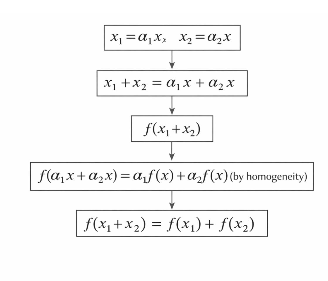
Figure 2.19: Derivation of additivity from homogeneity under continuity assumptions. |
2.25 Implications for Linear System Theory
The derivation above demonstrates that in continuous systems, homogeneity alone is sufficient to guarantee additivity. As a result, additivity and homogeneity are not independent conditions in this special case. Either property can imply the other when continuity is assumed.
This equivalence is particularly relevant in biomedical imaging and signal processing, where systems are often modeled as continuous and smooth. Under these assumptions, verifying one linearity condition may be enough to justify the use of linear system theory. This simplification supports the widespread application of superposition, Fourier analysis, and reconstruction algorithms in medical imaging.
Understanding when and why these properties are equivalent helps clarify the theoretical foundations of linear modeling. It also highlights the importance of continuity assumptions when applying mathematical abstractions to real-world imaging systems.
2.26 Independence of Homogeneity
Although additivity and homogeneity together define linearity, additivity alone does not guarantee homogeneity. This can be demonstrated using a counterexample from complex-valued functions. Such examples are important because they show why both properties must be explicitly verified when testing whether a system is linear.
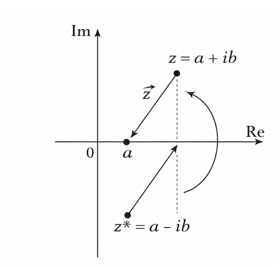
Figure 2.20: Complex conjugation preserves additivity but violates homogeneity for complex scalars. |
Consider the function
\[f(z) = z^*\]where (z = a + ib) is a complex number and (z^* = a - ib) denotes its complex conjugate.
This function maps each complex number to its conjugate and is commonly encountered in complex analysis and signal processing.
To test additivity, let (z_1) and (z_2) be complex numbers. Then
\[f(z_1 + z_2) = (z_1 + z_2)^* = z_1^* + z_2^* = f(z_1) + f(z_2).\]This confirms that the function satisfies additivity, since the conjugate of a sum equals the sum of the conjugates.
However, homogeneity does not hold for this function. For a complex scalar $\alpha$,
\[f(\alpha z) = (\alpha z)^* = \alpha^* z^*\]which is not equal to
\[\alpha z^* = \alpha f(z)\]unless $\alpha$ is real.
Because complex conjugation also conjugates the scalar, the scaling factor is altered.
This violation of homogeneity demonstrates that additivity alone is insufficient to establish linearity.
This example shows that a system can be additive without being homogeneous. Therefore, additivity does not imply homogeneity, and both conditions must be checked independently when determining whether a system is linear.
2.27 Independence of Additivity
Homogeneity alone is also insufficient to guarantee linearity, as demonstrated by a counterexample involving real-valued functions. Consider the function
\(f(x) = \begin{cases} m_1 x, & \text{if } x \text{ is rational}, \\ m_2 x, & \text{if } x \text{ is irrational}. \end{cases}\) where $m_1$ and $m_2$ are rational constants with $m_1 \ne m_2$. This function behaves differently depending on whether the input is rational or irrational.
Assume that the scalar domain consists only of rational numbers. Under rational scaling, the rationality or irrationality of a number does not change. Therefore, for any rational scalar $\alpha$,
\[f(\alpha x) = \alpha f(x)\]which confirms that the function satisfies homogeneity under this restricted scalar domain.
However, additivity fails for this function. Consider two irrational numbers $x_1$ and $x_2$ whose sum is rational. Then,
\[f(x_1 + x_2) = m_1(x_1 + x_2)\]since $x_1 + x_2$ is rational. On the other hand,
\[f(x_1) + f(x_2) = m_2 x_1 + m_2 x_2 = m_2(x_1 + x_2)\]Because $m_1 \ne m_2$, these expressions are not equal, and additivity is violated.
This example demonstrates that homogeneity does not imply additivity. A system may scale inputs correctly while failing to preserve sums, which disqualifies it from being linear.
2.28 Implications for Testing Linearity
The counterexamples presented above establish that additivity and homogeneity are logically independent properties in general. Neither condition alone is sufficient to guarantee linearity unless additional assumptions, such as continuity, are imposed. As a result, both properties must be explicitly verified when analyzing an unknown system.
In biomedical signal processing and medical imaging, assumptions of linearity are often made to simplify analysis and computation. However, these assumptions must be justified carefully, especially when dealing with nonlinear tissue responses, hardware limitations, or signal-dependent effects. Understanding the independence of additivity and homogeneity helps prevent incorrect modeling assumptions.
By rigorously testing both conditions, engineers and scientists ensure that linear system theory is applied only when appropriate. This rigor underpins reliable image reconstruction, signal analysis, and system design in modern bioimaging applications.
2.29 Relative Linearity
In many practical systems, the apparent behavior of a system may not look strictly linear when absolute input and output values are considered. This discrepancy arises because real-world systems often include offsets, biases, or baseline values that shift the output independently of the input. While the system may seem nonlinear under these conditions, it can behave linearly when examined in terms of relative changes—that is, changes from a reference point rather than absolute values.
To formalize this idea, consider the system’s input-output relationship defined in a specific coordinate system. Let the input change by $\Delta x_1(t)$, producing a corresponding output change $\Delta y_1(t)$, such that
\[\Delta y_1(t) = L[\Delta x_1(t)].\]Similarly, a second input change $\Delta x_2(t)$ produces
\[\Delta y_2(t) = L[\Delta x_2(t)].\]If the system satisfies linearity for these relative changes, then any weighted combination of the input changes also produces a proportional combination of output changes:
\[\alpha \Delta y_1(t) + \beta \Delta y_2(t) = L[\alpha \Delta x_1(t) + \beta \Delta x_2(t)].\]where $\alpha$ and $\beta$ are scalar weights.
This approach essentially redefines the linear system around a reference operating point, often referred to as the system’s nominal state. By focusing on deviations from this reference, the system behaves according to the superposition principle, even if the absolute input-output function includes an intercept or other nonlinear baseline behavior. The key insight is that linearity can be meaningful in terms of relative changes, rather than absolute values.
In medical imaging, relative linearity is particularly useful. Imaging devices often have baseline offsets or background signals, such as dark current in optical detectors or baseline voltage in MRI receivers. By analyzing changes in signals relative to these baselines, rather than raw absolute measurements, the system can be treated as effectively linear. This simplifies reconstruction algorithms, calibration procedures, and quantitative analyses. For example, in functional MRI (fMRI), relative changes in signal intensity are used to infer brain activity rather than absolute signal values. Similarly, in CT or ultrasound imaging, analyzing contrast or intensity changes relative to tissue background allows linear models to guide reconstruction and processing, even when absolute signals include offsets.
By adopting a relative perspective, engineers and clinicians can apply linear system theory more broadly and leverage the associated mathematical tools, such as superposition, convolution, and Fourier analysis. This makes it possible to model, analyze, and interpret imaging data effectively, even when the underlying physical system exhibits nonlinear offsets in absolute terms.
2.30 Voltage–Current Relationships in Electrical Components
Understanding how basic electrical components respond to voltage and current is fundamental for analyzing circuits in biomedical imaging systems. The voltage–current (V–I) relationships define how each component behaves under different electrical conditions, and these relationships also illustrate the concept of linearity in physical systems. Resistors, capacitors, and inductors, while each having distinct characteristics, are widely used in imaging equipment to regulate and stabilize electrical signals.
2.30.1 Resistors
A resistor is the simplest linear electrical component, and its behavior is governed by Ohm’s law. The relationship between voltage $v$ across a resistor and the current $i$ through it is given by
\[v = iR\]where $R$ is the resistance. This equation shows that the voltage is directly proportional to the current. Equivalently, one can express the current as a function of voltage:
\[i = \frac{v}{R}.\]Whether voltage is treated as a function of current or vice versa, the relationship remains clearly linear, as the slope of the V–I curve is constant. In biomedical imaging systems, resistors are used to control signal amplitudes, set biasing conditions in sensors, and limit current to protect sensitive components. Their predictable linear behavior makes them essential for precise and stable circuit operation.
2.30.2 Capacitors
A capacitor stores electrical charge and exhibits a V–I relationship that depends on the time rate of change of current or voltage. The voltage across a capacitor is related to the accumulated charge by
\[v(t) = \frac{1}{C} \int_{t_0}^{t} i(\tau)\, d\tau + v(t_0)\]where $C$ is the capacitance, $i(\tau)$ is the current, and $v(t_0)$ is the initial voltage at the start of the integration period. Conversely, the current through a capacitor is related to the rate of change of voltage:
\[i(t) = C \frac{dv(t)}{dt}.\]These equations reflect the fact that a capacitor accumulates electrical charge over time, and the current depends on how rapidly the voltage changes. Capacitors are widely used in medical imaging electronics to stabilize power supplies and smooth analog signals before they are converted into digital data. For example, in CT or MRI systems, capacitors filter high-frequency noise and provide consistent voltage levels to sensitive detectors and amplifiers, ensuring accurate measurements and reducing artifacts in images.
2.30.3 Inductors
An inductor opposes sudden changes in current, storing energy in a magnetic field. Its V–I relationships are complementary to those of capacitors. The voltage across an inductor is proportional to the rate of change of current:
\[v(t) = L \frac{di(t)}{dt}\]where $L$ is the inductance. Conversely, the current through an inductor depends on the integral of voltage over time:
\[i(t) = \frac{1}{L} \int_{t_0}^{t} v(\tau)\, d\tau + i(t_0)\]Unlike capacitors, which resist sudden voltage changes, inductors resist sudden changes in current. This property allows the current to build gradually rather than instantaneously, which helps smooth and stabilize electrical signals. In medical imaging equipment such as MRI machines, inductors are crucial for maintaining steady currents in coils and amplifiers, preventing spikes or fluctuations that could distort signals or damage sensitive hardware.
2.30.4 Summary of V–I Behavior
Resistors, capacitors, and inductors illustrate different aspects of electrical linearity. Resistors exhibit direct proportionality between voltage and current, capacitors relate current to the derivative of voltage (or voltage to integrated current), and inductors relate voltage to the derivative of current (or current to integrated voltage). In biomedical imaging systems, these components work together to regulate, filter, and stabilize signals, ensuring high-quality, accurate imaging while protecting sensitive electronic equipment.
2.31 Shift-Invariant Linear Systems
A shift-invariant linear system is a system in which a shift in the input signal results in an equivalent shift in the output signal, without changing the shape or characteristics of the response. In other words, the system’s behavior does not depend on the absolute position of the input in time or space; it responds in the same way regardless of when or where the input occurs. Mathematically, if the system is represented by an operator $L$ and produces an output $w(t)$ for an input $v(t)$, shift invariance is expressed as
\[v(t - \tau) \xrightarrow{L} w(t - \tau)\]or equivalently,
\[L[v(t - \tau)] = w(t - \tau)\]where $\tau$ is the shift in the input signal.
A real-world example of a shift-invariant system is an audio amplifier. If an audio signal is delayed by a few seconds before being input, the amplified output is the same waveform delayed by the same amount. The amplifier does not change the tone or amplitude of the signal based on the time of arrival; it treats all inputs consistently, simply producing a shifted version of the output.
Shift invariance provides several benefits in medical imaging. Imaging systems often measure signals sequentially in time or across spatial coordinates, such as the acquisition of slices in a a CT scanner or echoes in MRI. Shift invariance ensures that the system processes each part of the signal consistently, making the response predictable and allowing image reconstruction algorithms to assume uniform behavior across time or space. This property is crucial for techniques like convolution-based filtering, deblurring, and tomographic reconstruction, which rely on the output being a shifted version of the input when the input itself is shifted.
Shift invariance can also be expressed in the spatial or general functional domain. For a function $f(x)$ processed by a system to produce output $g(x)$, the property is written as
\[f(x - a) \xrightarrow{L} g(x - a)\]where a shift a in the input produces the same shift in the output. This general form applies to both time-domain signals and spatial-domain imaging. For instance, in MRI, moving the imaging slice slightly along one axis shifts the measured signals in a predictable way without altering their shape, which is a direct manifestation of spatial shift invariance.
Shift invariance is sometimes referred to as temporal invariance when applied in the time domain or spatial invariance when applied in imaging coordinates. In all cases, the key idea is that the system’s behavior depends only on the form of the input, not its location. This property greatly simplifies analysis and processing because linear operations, such as convolution and filtering, can be applied universally across all parts of the signal or image.
In summary, shift-invariant linear systems provide a foundation for predictable, consistent signal processing in both time and space. Their properties allow engineers to design algorithms for filtering, reconstruction, and analysis that can be applied uniformly across an entire dataset, which is critical for producing high-quality, accurate medical images.
2.32 Nonlinear Systems
A nonlinear system is a system in which the output is not directly proportional to the input, meaning that the principles of additivity and homogeneity no longer apply. Unlike linear systems, nonlinear equations are often more difficult to solve, and in many cases it is impossible to find exact analytical solutions. Nonlinear systems can exhibit behaviors that are counterintuitive or unpredictable, including chaos, solitons, and singularities, which do not appear in linear systems.
Modern computing has made it possible to study and simulate nonlinear systems numerically, providing insight into their complex behavior even when exact solutions cannot be obtained. Nonlinear systems are encountered across science and engineering, from fluid dynamics and weather modeling to biological population dynamics and biomedical imaging signal processing. These systems can exhibit emergent patterns, where simple underlying rules generate highly intricate or unpredictable outcomes.
A classical example of a nonlinear system is the logistic map, a mathematical model commonly used in population dynamics. The logistic map is expressed as
\[x_{n+1} = r \, x_n \, (1 - x_n),\]where $x_n$ represents the population at generation $n$ (normalized to the maximum capacity of the environment), and $r$ is the growth rate parameter. The term $1 - x_n$ accounts for environmental limitations: as the population approaches the maximum capacity, growth slows due to scarcity of resources.
The logistic map demonstrates how complex behaviors emerge from a simple nonlinear equation. Depending on the value of the growth rate rrr, the population may stabilize at a fixed value, oscillate between multiple values, or exhibit chaotic fluctuations where small changes in initial conditions lead to vastly different outcomes. This model reflects how natural systems regulate themselves and illustrates the rich variety of patterns that can arise in nonlinear systems.
Nonlinear dynamics have broad implications beyond ecology. In biomedical engineering, nonlinear models are used to describe neural network activity, cardiac rhythms, and even the nonlinear response of imaging systems at extreme operating ranges. Understanding the principles of nonlinear systems allows engineers and scientists to anticipate unexpected behavior, design robust control strategies, and interpret complex signals that would be misrepresented by linear approximations.
In summary, while nonlinear systems are mathematically more challenging than linear systems, they capture the richness and complexity of real-world phenomena. Simple nonlinear rules, like those in the logistic map, can produce stability, periodicity, or chaos, revealing how complex behavior emerges naturally from simple equations.
2.33 Chaotic Behavior
Chaos in mathematical systems refers to deterministic behavior that is extremely sensitive to initial conditions. In chaotic systems, even small changes at the start can lead to dramatically different outcomes over time. A common example is long-term weather forecasting: despite the underlying physics being deterministic, small measurement errors in the initial state can produce widely divergent predictions after a few days, making forecasts unreliable beyond a certain time horizon.
Graphs of chaotic systems, such as iterations of the logistic map, often display complex, seemingly random patterns, even though they arise from simple deterministic rules. Chaos is an important concept in nonlinear dynamics because it highlights how predictability can break down, even when the system is governed by known equations. Understanding chaotic behavior is critical in modeling natural systems, including biological rhythms, cardiac signals, and population dynamics, where small fluctuations can have large effects.
2.34 Biological and Artificial Neurons
A biological neuron is a specialized cell that processes and transmits information in the nervous system. It collects incoming signals through branched structures called dendrites, which receive chemical or electrical inputs from other neurons. These inputs are integrated in the cell body (soma). While small individual inputs may have little or no effect, when the combined inputs exceed a certain threshold, the neuron fires an action potential, sending an electrical impulse along the axon to the synapses. At the synapses, this signal communicates with the next neuron, propagating information through the network.
This threshold-based behavior allows the nervous system to filter out noise and respond only to meaningful stimuli. From a mathematical perspective, biological neurons can be modeled as artificial neurons, which sum their inputs, apply a non-linear activation function, and produce an output if the threshold is exceeded. This abstraction forms the basis of modern neural networks, linking biological principles to computational models.
2.35 Deep Neural Networks (DNNs)
Deep neural networks (DNNs) are composed of multiple layers of artificial neurons, organized hierarchically. Each layer learns increasingly abstract feature representations from the input data. The first layer might learn simple features, such as edges or colors in an image, while subsequent layers combine these features to recognize more complex patterns, such as shapes, objects, or tissue structures in medical images.
Training a DNN involves adjusting the weights of connections between neurons based on the difference between the predicted output and the true output, a process called backpropagation. Layered learning enables the network to identify hierarchical structures in data, making DNNs extremely effective at tasks that require pattern recognition.
In the real world, DNNs are widely used in image and signal processing applications. In medical imaging, DNNs assist in detecting tumors in MRI scans, segmenting organs in CT images, and enhancing low-quality ultrasound data. Outside medicine, DNNs power autonomous vehicles, speech recognition, and facial recognition, demonstrating the broad utility of hierarchical feature learning.
By modeling both biological and artificial neural networks, engineers and researchers gain insight into how complex patterns and meaningful information can be extracted from noisy or high-dimensional data. This principle underlies much of modern biomedical imaging and AI-assisted diagnostics.